Introduction by Example

We shortly introduce the datasets provided by ℋ²GB and the versatile UnifiedGT framework through self-contained examples.

For an introduction to Graph Machine Learning, we refer the interested reader to the Stanford CS224W: Machine Learning with Graphs lectures.

At its core, ℋ²GB provides the following main features:

Heterophilic and Heterogeneous Graph Datasets

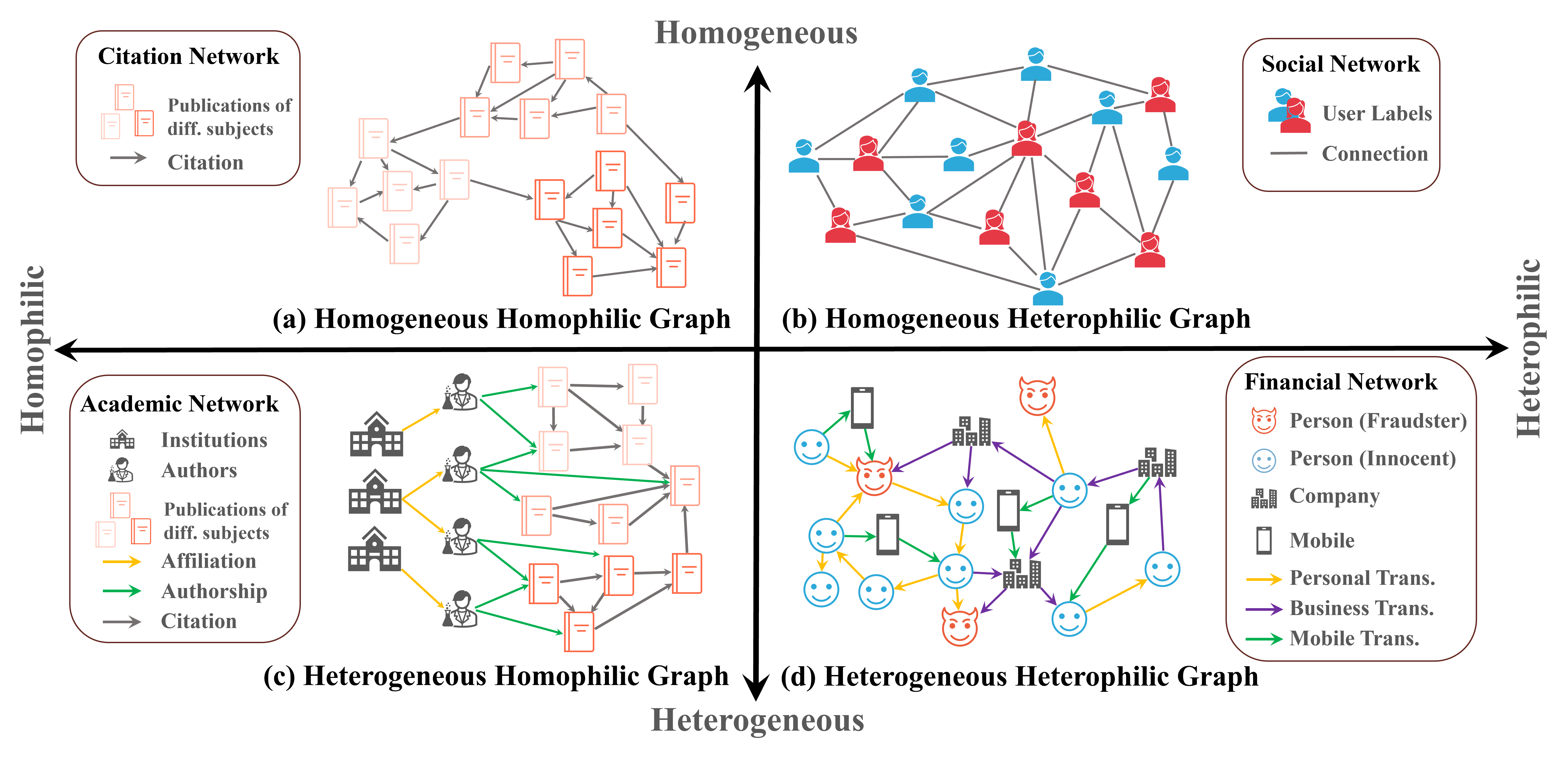
Many real-world graphs, such as academic networks, social networks and financial networks, frequently present challenges for graph learning due to heterophily, where connected nodes may have dissimilar labels and attributes, and heterogeneity, where multiple types of entities and relations among the graphs are embodied by various types of nodes and edges. Each of these two properties can significantly impede the performance of graph learning models. While there have been advancements in handling graph with heterophily and heterogeneity seperately, there is a lack of research on learning on graphs with both of these two properties, which many real-world graphs have. For example, financial networks (subfigure (d)) are both heterophilic and heterogeneous. Different node types (person, business, etc.) and edge types (wire transfer, credit card transaction, etc.) exist, making the graph heterogeneous. The class labels of fraudsters differ from those of their innocent neighbors, making the graph heterophilic. There are also many graphs from other domains that are both heterophilic and heterogeneous, such as networks from e-commerce, academia, and cybersecurity.

In ℋ²GB, we provide 9 diverse real-world datasets across 5 domains – academia, finance, e-commerce, social science, and cybersecurity.

Access Datasets

Datasets can be easily loaded through the create_dataset() method. ℋ²GB is gloablly configured by an internal config tree. In the following example, we demonstrate that by loading an external mag-year-MLP configuration file, you are able to access the mag-year dataset.

Note

It’s also possible to directly modify the attributes inside the cfg variable, without the need to load an external configuration file.

import argparse
import H2GB
from H2GB.graphgym.config import cfg, set_cfg, load_cfg
from H2GB.graphgym.loader import create_dataset

# Load cmd line args
parser = argparse.ArgumentParser(description='H2GB')
parser.add_argument('--cfg', dest='cfg_file', type=str, required=True,
                    help='The configuration file path.')
parser.add_argument('opts', default=None, nargs=argparse.REMAINDER,
                    help='See graphgym/config.py for remaining options.')

args = parser.parse_args(["--cfg", "configs/mag-year/mag-year-MLP.yaml"])
# Load config file
set_cfg(cfg)
load_cfg(cfg, args)

dataset = create_dataset()
data = dataset[0]
print(dataset)
print(data)

Running Experiments

Experiments are configued by configuration files available in /configs and are easy to reproduce. Before reproducing experiments, you will need to firstly specify the dataset and log locations by editing the config file provided under /configs/{dataset_name}/. An example configuration is

......
out_dir: ./results/{Model Name} # Put your log output path here
dataset:
dir: ./data # Put your input data path here
......

Create empty folders for storing the dataset and results. Dataset download will be automatically initiated if dataset is not found under the specified location.

For convenience, a script file is created to run the experiment with specified configuration. For instance, you can edit and run the interactive_run.sh to start the experiment.

# Assuming you are located in the H2GB repo
chmox +x ./run/interactive_run.sh
./run/interactive_run.sh

You can also directly enter this command into your terminal:

python -m H2GB.main --cfg {Path to Your Configs} name_tag {Custom Name Tag}

For example, the following command is to run MLP model experiment for oag-cs dataset.

python -m H2GB.main --cfg configs/oag-cs/oag-cs-MLP.yaml name_tag MLP

Note

ℋ²GB currently only supports CPU or single-GPU training. You can specify the device entry in the configuration files as follow. The default value of device is auto, which will automatically detect GPU device and select the GPU with the least memory usage.

......
device: cpu/cuda/cuda:0/auto
......

Make Use of Modular Ingredients

In the following, we list out the available modular ingredients provided in UnifiedGT framework.

Graph Sampling	Graph Encoding	Graph Attention	Attention Masking	Feedforward Networks (FFNs)
Neighbor Sampling	Node2Vec Embedding	Plain Attention	None	Single
GraphSAINT Sampling	Metapath2Vec Embedding	Cross-type Heterogeneous Attention	Direct Neighbor Mask	Type-specific
HGSampling	Knowledge Graph Embedding
	Masked Label Embedding

You can make use of each component by specifying the configuration files. We list a few examples in the following subsections.

Graph Sampling

For example, to select different graph sampler, you only need to modify the train.sampler, train.neighbor_sizes and val.sampler. To use a neighbor sampler, set as the following

......
train:
    sampler: hetero_neighbor
    neighbor_sizes: [20, 15, 10]
......
val:
    sampler: hetero_neighbor
......

Graph Encoding

To select different graph encoding method, you only need to modify the dataset.node_encoder_name. To use a Node2Vec embedding, set as the following

......
dataset:
    node_encoder_name: Raw+Hetero_Node2Vec
......

You can even combine multiple graph encoding together, for example, combining masked label embedding and Metapath2Vec together

......
dataset:
    node_encoder_name: Raw+Hetero_Label+Hetero_Metapath
......

Graph Attention

To select different graph encoding method, you can modify the gt.layer_type. We have several graph transformer examples that made use of different graph attention, such as in GraphTrans and Gophormer:

......
gt:
    layer_type: TorchTransformer/SparseNodeTransformer
......

Attention Masking

You can apply different attention masking method by changing the gt.attn_mask.

......
gt:
    attn_mask: none/Edge/kHop
......

Feedforward Networks (FFNs)

We provide two choices in the gt.ffn, corresponding to single FFN and type-specific FFN.

......
gt:
    ffn: Single/Type
......

Metric Selection

As our UnifiedGT framework provides a unified evaluator, you can conveniently select different evaluation metric depends on the demand of your custom dataset. You just need to specify metric_best in your configuration file. For example metric_best: accuracy. We have provided many choices of evaluation metrics, which is defined in /H2GB/logger.py. We defined 3 scenarios of downstream tasks, which are binary classification, multi-class classification and multi-label classification. We details the definition of these three scenarios and their correpsonding supported metrics in the following subsections.

Binary Classification

The goal of binary classification is to categorize data into one of two classes or categories. The true label is an integer containing only \(0`\) and \(1\). The prediction from the model is usually a real number which would pass through a sigmoid function to convert to a probability that it belongs to the positive class.

We support accuracy, precision, recall, f1, macro-f1, micro-f1, and auc for this scenario.

Multi-class Classification

The goal of multi-class classification is to categorize data into more than two classes. The true label is an integer between \(0\) and \(C-1\). The prediction from the model is usually a vector of \(C\) real number which would pass through a softmax function to convert to a probability that it belongs to a certain class.

We support accuracy, f1, and micro-f1 for this scenario.

Multi-label Classification

Multi-label classification assigns multiple labels to an instance, allowing it to belong to more than one category simultaneously. The true label is an a vector of \(C\) binary number representing what label it has. The prediction from the model is usually \(C\) real number which would pass through a sigmoid function respectively to convert to a probability that it contains a certain label.

We support accuracy, f1, auc, and ap for this scenario.